十大排序算法

Posted on 2021-11-20 Edited on 2024-07-22 In 数据结构与算法 , 数据结构 Views: Word count in article: 17k Reading time ≈ 16 mins.

1、排序算法说明

排序的定义

对一序列对象根据某个关键字进行排序。

相关术语说明

稳定：如果a原本在b前面，而a=b，排序之后a仍然在b的前面。
不稳定：如果a原本在b的前面，而a=b，排序之后a可能会出现在b的后面。
内排序：所有排序操作都在内存中完成。
外排序：由于数据太大，因此把数据放在磁盘中，而排序通过磁盘和内存的数据传输才能进行。
时间复杂度： 一个算法执行所耗费的时间。
空间复杂度：运行完一个程序所需内存的大小。

十大排序算法对比

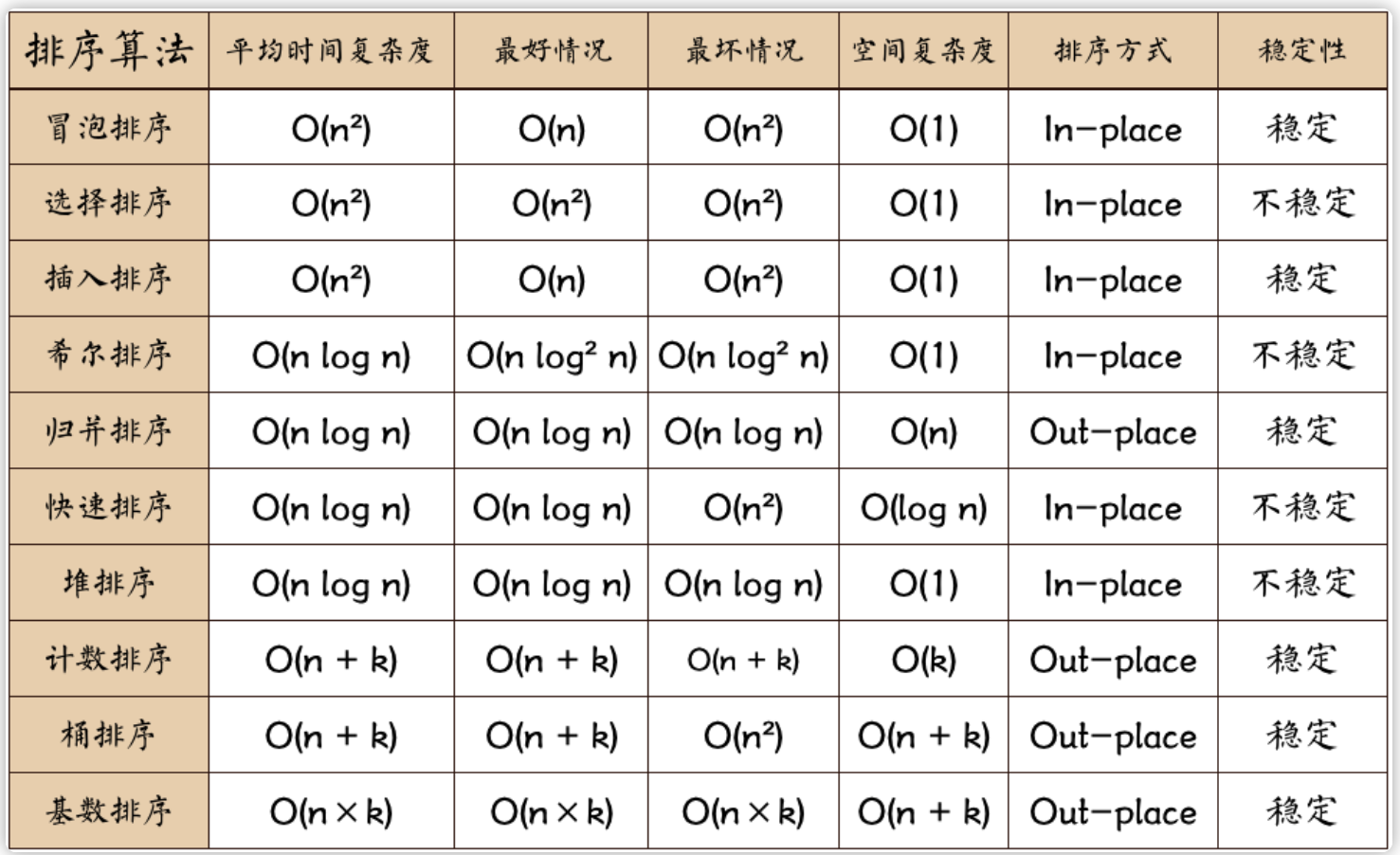
n：数据规模。
k：”桶”的个数。
In-place：占用常数内存，不占用额外内存。
Out-place：占用额外内存。

十大排序算法分类

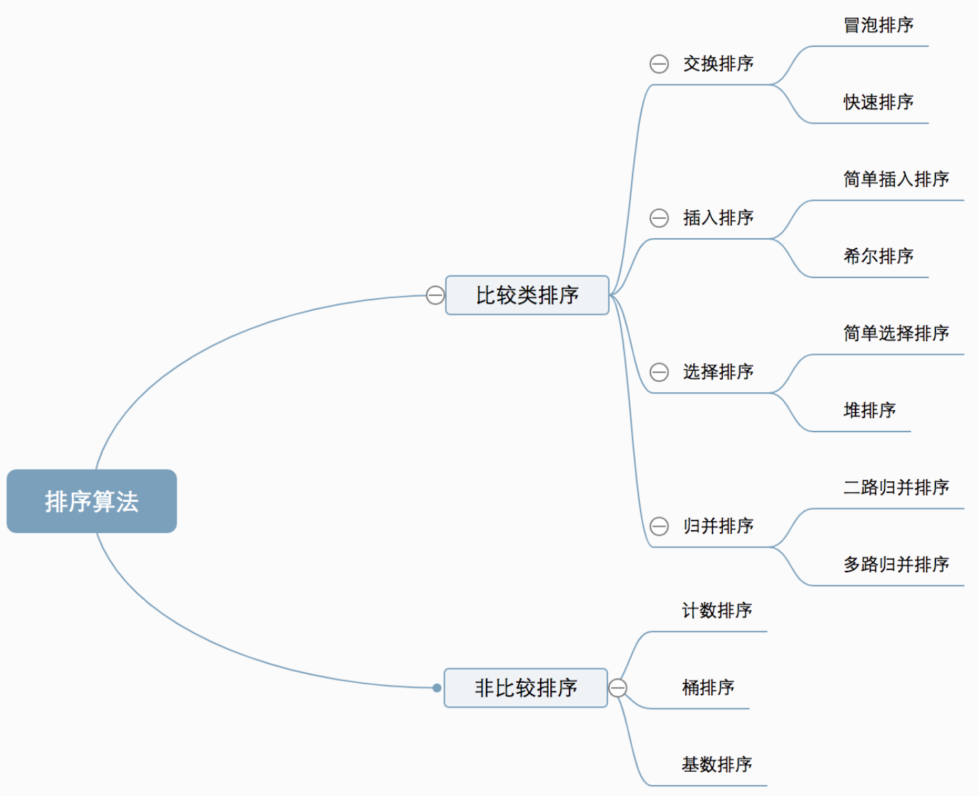
比较类排序：通过比较来决定元素间的相对次序，由于其时间复杂度不能突破O(nlogn)，因此也称为非线性时间比较类排序。即在排序的最终结果里，元素之间的次序依赖于它们之间的比较。每个数都必须和其他数进行比较，才能确定自己的位置。比较排序的优势是，适用于各种规模的数据，也不在乎数据的分布，都能进行排序。可以说，比较排序适用于一切需要排序的情况。
非比较类排序：不通过比较来决定元素间的相对次序，它可以突破基于比较排序的时间下界，以线性时间运行，因此也称为线性时间非比较类排序。即非比较排序是通过确定每个元素之前，应该有多少个元素来排序。针对数组arr，计算arr[i]之前有多少个元素，则唯一确定了arr[i]在排序后数组中的位置。算法时间复杂度O(n)，非比较排序时间复杂度低，但由于非比较排序需要占用空间来确定唯一位置，所以对数据规模和数据分布有一定的要求。

2、十大排序算法

2.1 冒泡排序

冒泡排序是一种简单的排序算法。它重复地走访过要排序的数列，一次比较两个元素，如果它们的顺序错误就把它们交换过来。走访数列的工作是重复地进行直到没有再需要交换，也就是说该数列已经排序完成。这个算法的名字由来是因为越小的元素会经由交换慢慢”浮”到数列的顶端。

比较相邻的元素。如果第一个比第二个大，就交换它们两个；
对每一对相邻元素作同样的工作，从开始第一对到结尾的最后一对，这样在最后的元素应该会是最大的数；
针对所有的元素重复以上的步骤，除了最后一个；
重复步骤1~3，直到排序完成。

public static int[] bubbleSort(int[] arr) {
    int temp = 0;
    for (int i = 0; i < arr.length - 1; i++) {
        for (int j = 0; j < arr.length - i - 1; j++) {
            if (arr[j] > arr[j + 1]) {
                temp = arr[j];
                arr[j] = arr[j + 1];
                arr[j + 1] = temp;
            }
        }
    }
    return arr;
}

2.2 选择排序

选择排序(Selection-sort)是一种简单直观的排序算法。它的工作原理：首先在未排序序列中找到最小（大）元素，存放到排序序列的起始位置，然后，再从剩余未排序元素中继续寻找最小（大）元素，然后放到已排序序列的末尾。以此类推，直到所有元素均排序完毕。是表现最稳定的排序算法之一，因为无论什么数据进去都是O(n2)的时间复杂度，所以用到它的时候，数据规模越小越好。

初始状态：无序区为R[1..n]，有序区为空；
第i趟排序(i=1,2,3…n-1)开始时，当前有序区和无序区分别为R[1..i-1]和R(i..n）。该趟排序从当前无序区中-选出关键字最小的记录 R[k]，将它与无序区的第1个记录R交换，使R[1..i]和R[i+1..n)分别变为记录个数增加1个的新有序区和记录个数减少1个的新无序区；
n-1趟结束，数组有序化了。

public static int[] selectSort(int[] arr) {
    int temp;
    int minIndex;
    for (int i = 0; i < arr.length - 1; i++) {
        minIndex = i;
        for (int j = i + 1; j < arr.length; j++) {
            // 寻找最小的数
            if (arr[j] < arr[i]) {
                // 将最小数的索引保存
                minIndex = j;
            }
        }
        temp = arr[i];
        arr[i] = arr[minIndex];
        arr[minIndex] = temp;
    }
    return arr;
}

2.3 插入排序

是一种简单直观的排序算法。它的工作原理是通过构建有序序列，对于未排序数据，在已排序序列中从后向前扫描，找到相应位置并插入。插入排序在实现上，通常采用in-place排序（即只需用到O(1)的额外空间的排序），因而在从后向前扫描过程中，需要反复把已排序元素逐步向后挪位，为最新元素提供插入空间。

从第一个元素开始，该元素可以认为已经被排序；
取出下一个元素，在已经排序的元素序列中从后向前扫描；
如果该元素（已排序）大于新元素，将该元素移到下一位置；
重复步骤3，直到找到已排序的元素小于或者等于新元素的位置；
将新元素插入到该位置后；
重复步骤2~5。

public static int[] insertSort(int[] arr) {
    // 需要插入的数
    int insertVal;
    // 该数需要插入数组的索引
    int insertIndex;
    for (int i = 1; i < arr.length; i++) {
        insertVal = arr[i];
        insertIndex = i - 1;
        while (insertIndex >= 0 && insertVal < arr[insertIndex]) {
            arr[insertIndex + 1] = arr[insertIndex];
            insertIndex--;
        }
        arr[insertIndex + 1] = insertVal;
    }
    return arr;
}

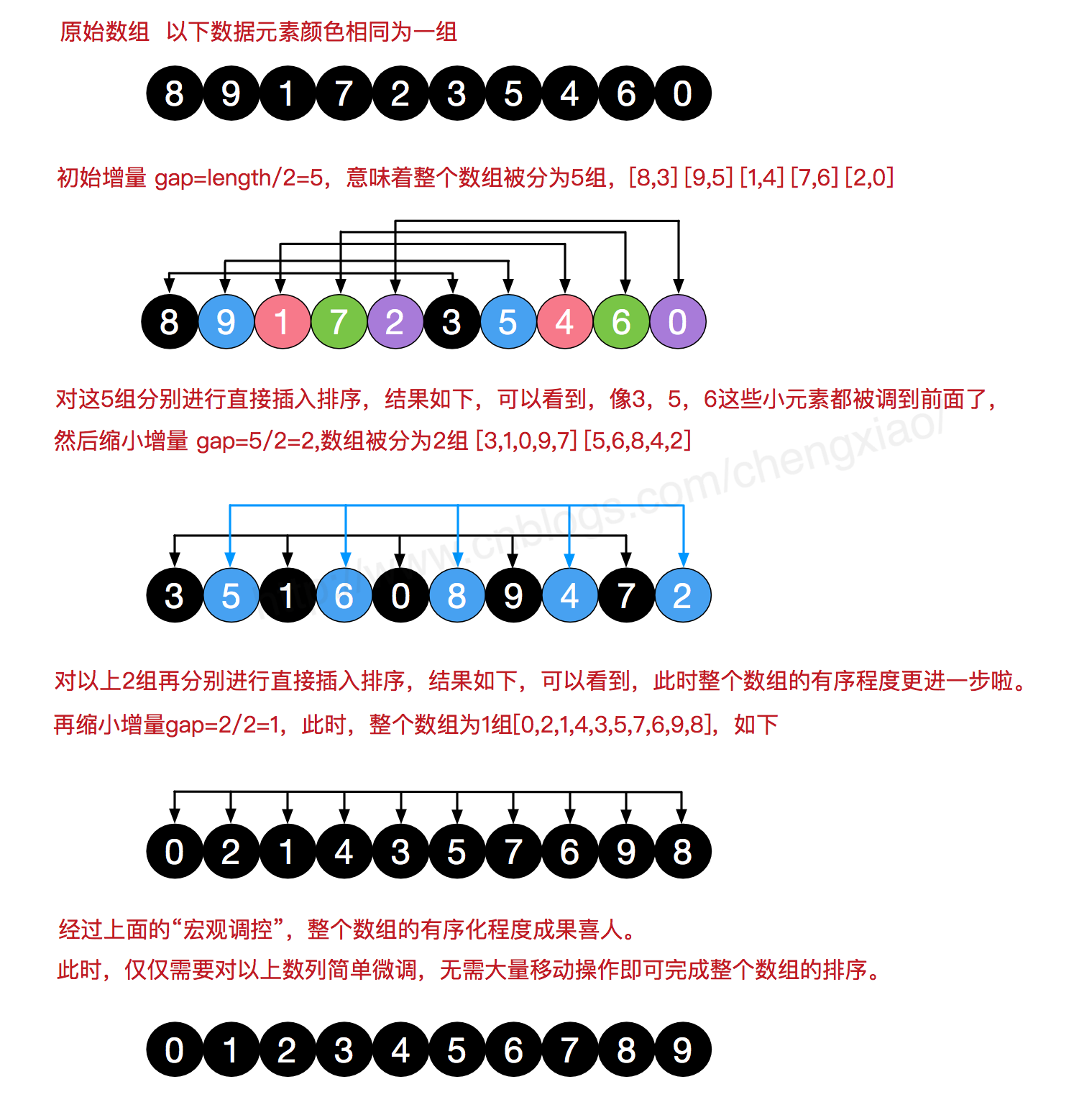
2.4 希尔排序

希尔排序也是一种插入排序，它是简单插入排序经过改进之后的一个更高效的版本，也称为缩小增量排序，同时该算法是冲破O(n2）的第一批算法之一。它与插入排序的不同之处在于，它会优先比较距离较远的元素。希尔排序又叫缩小增量排序。希尔排序是把记录按下表的一定增量分组，对每组使用直接插入排序算法排序；随着增量逐渐减少，每组包含的关键词越来越多，当增量减至1时，整个文件恰被分成一组，算法便终止。先将整个待排序的记录序列分割成为若干子序列分别进行直接插入排序，具体算法描述：

选择一个增量序列t1，t2，…，tk，其中ti>tj，tk=1；
按增量序列个数k，对序列进行k趟排序；
每趟排序，根据对应的增量ti，将待排序列分割成若干长度为m的子序列，分别对各子表进行直接插入排序。仅增量因子为1时，整个序列作为一个表来处理，表长度即为整个序列的长度。

public static int[] ShellSort(int[] arr) {
    int len = arr.length;
    int gap = len / 2;
    // 需要插入的数
    int insertVal;
    // 该数需要插入数组的索引
    int insertIndex;
    while (gap > 0) {
        for (int i = gap; i < len; i++) {
            insertVal = arr[i];
            insertIndex = i - gap;
            while (insertIndex >= 0 && insertVal < arr[insertIndex]) {
                arr[insertIndex + gap] = arr[insertIndex];
                insertIndex -= gap;
            }
            arr[insertIndex + gap] = insertVal;
        }
        gap /= 2;
    }
    return arr;
}

2.5 归并排序

归并排序是建立在归并操作上的一种有效的排序算法。该算法是采用分治法（Divide and Conquer）的一个非常典型的应用，它是一种稳定的排序方法。将已有序的子序列合并，得到完全有序的序列。即先使每个子序列有序，再使子序列段间有序。若将两个有序表合并成一个有序表，称为2-路归并。和选择排序一样，归并排序的性能不受输入数据的影响，但表现比选择排序好的多，因为始终都是O(nlog n）的时间复杂度。代价是需要额外的内存空间。

把长度为n的输入序列分成两个长度为n/2的子序列；
对这两个子序列分别采用归并排序；
将两个排序好的子序列合并成一个最终的排序序列。

public static int[] merge(int[] nums, int left, int right) {
    int mid = left + ((right - left) >> 1);
    if (left < right) {
        merge(nums, left, mid);
        merge(nums, mid + 1, right);
        mergeSort(nums, left, mid, right);
    }
    return nums;
}

public static void mergeSort(int[] nums, int left, int mid, int right) {
    int[] temp = new int[right - left + 1];
    int t = 0;
    int i = left;
    int j = mid + 1;
    while (i <= mid && j <= right) {
        if (nums[i] < nums[j]) {
            temp[t++] = nums[i++];
        } else {
            temp[t++] = nums[j++];
        }
    }
    // 把左边剩余的数移入数组
    while (i <= mid) {
        temp[t++] = nums[i++];
    }
    // 把右边剩余的数移入数组
    while (j <= right) {
        temp[t++] = nums[j++];
    }
    // 把新数组中的数覆盖nums数组
    for (int k = 0; k < t; k++) {
        nums[left + k] = temp[k];
    }
}

2.6 快速排序

快速排序的基本思想：通过一趟排序将待排记录分隔成独立的两部分，其中一部分记录的关键字均比另一部分的关键字小，则可分别对这两部分记录继续进行排序，以达到整个序列有序。快速排序使用分治法来把一个串（list）分为两个子串（sub-lists）。

从数列中挑出一个元素，称为”基准”（pivot）；
重新排序数列，所有元素比基准值小的摆放在基准前面，所有元素比基准值大的摆在基准的后面（相同的数可以到任一边）。在这个分区退出之后，该基准就处于数列的中间位置。这个称为分区（partition）操作；
递归地（recursive）把小于基准值元素的子数列和大于基准值元素的子数列排序。

public static void quickSort(int[] arr, int left, int right) {
    int i;
    int j;
    int flag;
    if (left < right) {
        i = left;
        j = right;
        flag = arr[i];
        while (i < j) {
            while (i < j && arr[j] >= flag) {
                j--;
            }
            arr[i] = arr[j];
            while (i < j && arr[i] < flag) {
                i++;
            }
            arr[j] = arr[i];
        }
        arr[i] = flag;
        quickSort(arr, left, i - 1);
        quickSort(arr, i + 1, right);
    }
}

2.7 堆排序

堆排序（Heapsort）是指利用堆这种数据结构所设计的一种排序算法。堆积是一个近似完全二叉树的结构，并同时满足堆积的性质：即子结点的键值或索引总是小于（或者大于）它的父节点。

将初始待排序关键字序列(R1,R2….Rn)构建成大顶堆，此堆为初始的无序区；
将堆顶元素R[1]与最后一个元素R[n]交换，此时得到新的无序区(R1,R2,……Rn-1)和新的有序区(Rn),且满足R[1,2…n-1]<=R[n]；
由于交换后新的堆顶R[1]可能违反堆的性质，因此需要对当前无序区(R1,R2,……Rn-1)调整为新堆，然后再次将R[1]与无序区最后一个元素交换，得到新的无序区(R1,R2….Rn-2)和新的有序区(Rn-1,Rn)。不断重复此过程直到有序区的元素个数为n-1，则整个排序过程完成。

public static int[] HeapSort(int[] array) {
    int len = array.length;
    if (len < 1) {
        return array;
    }
    // 从最后一个非叶子节点开始向上构造大顶堆
    for (int i = (len / 2 - 1); i >= 0; i--) {
        adjustHeap(array, i, len);
    }
    // 调整堆结构+交换堆顶元素与末尾元素
    for (int i = array.length - 1; i > 0; i--) {
        //将堆顶元素与末尾元素进行交换
        int temp = array[i];
        array[i] = array[0];
        array[0] = temp;
        // 重新对堆进行调整
        adjustHeap(array, 0, i);
    }
    return array;
}

/**
 * 调整使之成为最大堆
 */
public static void adjustHeap(int[] array, int i, int len) {
    // 先取出当前元素（父节点）的值，保存在临时变量
    int temp = array[i];
    // 得到左孩子
    int lChild = 2 * i + 1;
    while (lChild < len) {
        // 得到右孩子
        int rChild = lChild + 1;
        // 如果有右孩子结点，并且右孩子结点的值大于左孩子结点，则选取右孩子结点
        if (rChild < len && array[lChild] < array[rChild]) {
            lChild++;
        }
        // 如果父结点的值已经大于孩子结点的值，则直接结束
        if (temp >= array[lChild]) {
            break;
        } else {
            // 把孩子结点的值赋给父结点
            array[i] = array[lChild];
            // 选取孩子结点的左孩子结点,继续向下筛选
            i = lChild;
            lChild = 2 * lChild + 1;
        }
    }
    // 当while循环结束后，我们已经将以i为父结点的树的最大值，放在了最顶部(局部)
    array[i] = temp;
}

2.8 计数排序

计数排序的核心在于将输入的数据值转化为键存储在额外开辟的数组空间中。作为一种线性时间复杂度的排序，计数排序要求输入的数据必须是有确定范围的整数。

计数排序(Counting sort)是一种稳定的排序算法。计数排序使用一个额外的数组C，其中第i个元素是待排序数组A中值等于i的元素的个数。然后根据数组C来将A中的元素排到正确的位置。它只能对整数进行排序。

找出待排序的数组中最大和最小的元素；
统计数组中每个值为i的元素出现的次数，存入数组C的第i项；
对所有的计数累加（从C中的第一个元素开始，每一项和前一项相加）；
反向填充目标数组：将每个元素i放在新数组的第C(i)项，每放一个元素就将C(i)减去1。

public static int[] countSort(int[] array) {
    // 找出数组中的最大值
    int max = Integer.MIN_VALUE;
    for (int num : array) {
        max = Math.max(max, num);
    }
    // 初始化计数数组count
    int[] count = new int[max + 1];
    // 对计数数组各元素赋值
    for (int num : array) {
        count[num]++;
    }
    // 创建结果数组
    int[] result = new int[array.length];
    // 创建结果数组的起始索引
    int index = 0;
    // 遍历计数数组，将计数数组的索引填充到结果数组中
    for (int i = 0; i < count.length; i++) {
        while (count[i] > 0) {
            result[index++] = i;
            count[i]--;
        }
    }
    // 返回结果数组
    return result;
}

2.9 桶排序

桶排序是计数排序的升级版。它利用了函数的映射关系，高效与否的关键就在于这个映射函数的确定。桶排序可以看作是对计数排序的改进，计数排序对于数值在一定范围的整数数组可以进行排序，但是对于小数的数组却没有办法计数，这时候就要用到桶排序。

桶排序 (Bucket sort)的工作的原理：假设输入数据服从均匀分布，将数据分到有限数量的桶里，每个桶再分别排序（有可能再使用别的排序算法或是以递归方式继续使用桶排序进行排序。

public static float[] bucketSort(float[] arr) {
    // 新建一个桶的集合
    ArrayList<LinkedList<Float>> buckets = new ArrayList<LinkedList<Float>>();
    for (int i = 0; i < 10; i++) {
        // 新建一个桶，并将其添加到桶的集合中去。
        // 由于桶内元素会频繁地插入，所以选择 LinkedList 作为桶的数据结构
        buckets.add(new LinkedList<Float>());
    }
    // 将输入数据全部放入桶中并完成排序
    for (float data : arr) {
        int index = getBucketIndex(data);
        insertSort(buckets.get(index), data);
    }
    // 将桶中元素全部取出来并放入 arr 中输出
    int index = 0;
    for (LinkedList<Float> bucket : buckets) {
        for (Float data : bucket) {
            arr[index++] = data;
        }
    }
    return arr;
}

/**
 * 计算得到输入元素应该放到哪个桶内
 */
public static int getBucketIndex(float data) {
    // 这里例子写的比较简单，仅使用浮点数的整数部分作为其桶的索引值
    // 实际开发中需要根据场景具体设计
    return (int) data;
}

/**
 * 我们选择插入排序作为桶内元素排序的方法 每当有一个新元素到来时，我们都调用该方法将其插入到恰当的位置
 */
public static void insertSort(List<Float> bucket, float data) {
    ListIterator<Float> it = bucket.listIterator();
    boolean insertFlag = true;
    while (it.hasNext()) {
        if (data <= it.next()) {
            it.previous(); // 把迭代器的位置偏移回上一个位置
            it.add(data); // 把数据插入到迭代器的当前位置
            insertFlag = false;
            break;
        }
    }
    if (insertFlag) {
        bucket.add(data); // 否则把数据插入到链表末端
    }
}

public static void main(String[] args) {
    // 输入元素均在 [0, 10) 这个区间内
    float[] arr = new float[] { 0.12f, 2.2f, 8.8f, 7.6f, 7.2f, 6.3f, 9.0f, 1.6f, 5.6f, 2.4f };
    System.out.println(Arrays.toString(bucketSort(arr)));
}

桶排序中很重要的一步就是桶的设定了，我们必须根据输入元素的情况，选择一个恰当的 getBucketIndex算法，使得输入元素能够正确的放入对应的桶内，且保证输入数据能够尽量均匀的放入不同的桶内。
最糟糕的情况下，即所有的数据都放入了一个桶内，桶内自排序算法为插入排序，那么其时间复杂度就为 O(n ^ 2) 了。
其次，我们可以发现，区间划分的越细，即桶的数量越多，理论上分到每个桶中的元素就越少，桶内数据的排序就越简单，其时间复杂度就越接近于线性。
极端情况下，就是区间小到只有1，即桶内只存放一种元素，桶内的元素不再需要排序，因为它们都是相同的元素，这时桶排序差不多就和计数排序一样了。

2.10 基数排序

基数排序是桶排序的扩展，也是非比较的排序算法，对每一位进行排序，从最低位开始排序，复杂度为O(kn),为数组长度，k为数组中的数的最大的位数。

基数排序是按照低位先排序，然后收集；再按照高位排序，然后再收集；依次类推，直到最高位。有时候有些属性是有优先级顺序的，先按低优先级排序，再按高优先级排序。最后的次序就是高优先级高的在前，高优先级相同的低优先级高的在前。基数排序基于分别排序，分别收集，所以是稳定的。

public static int[] radixSort(int[] array) {
    if (array == null || array.length < 2) {
        return array;
    }
    // 先算出最大数的位数
    int max = array[0];
    for (int i = 1; i < array.length; i++) {
        max = Math.max(max, array[i]);
    }
    int maxDigit = 0;
    while (max != 0) {
        max /= 10;
        maxDigit++;
    }
    ArrayList<ArrayList<Integer>> bucketList = new ArrayList<>();
    for (int i = 0; i < 10; i++) {
        bucketList.add(new ArrayList<>());
    }
    for (int i = 0, n = 1; i < maxDigit; i++, n *= 10) {
        for (int j = 0; j < array.length; j++) {
            int num = array[j] / n % 10;
            bucketList.get(num).add(array[j]);
        }
        int index = 0;
        for (int j = 0; j < bucketList.size(); j++) {
            for (int k = 0; k < bucketList.get(j).size(); k++){
                array[index++] = bucketList.get(j).get(k);
            }
            bucketList.get(j).clear();
        }
    }
    return array;
}

3、LRU和LFU算法

3.1 LRU算法

LRU（Least Recently Used）是一种常见的页面置换算法，在计算中，所有的文件操作都要放在内存中进行，然而计算机内存大小是固定的，所以我们不可能把所有的文件都加载到内存，因此我们需要制定一种策略对加入到内存中的文件进项选择。
LRU的设计原理就是，当数据在最近一段时间经常被访问，那么它在以后也会经常被访问。这就意味着，如果经常访问的数据，我们需要然其能够快速命中，而不常访问的数据，我们在容量超出限制内，要将其淘汰。

要求实现LRUCache类：

LRUCache(int capacity)：以正整数作为容量capacity初始化LRU缓存。
int get(int key)：如果关键字 key 存在于缓存中，则返回关键字的值，否则返回-1。
void put(int key, int value)：如果关键字已经存在，则变更其数据值；如果关键字不存在，则插入该组[关键字-值]。当缓存容量达到上限时，它应该在写入新数据之前删除最久未使用的数据值，从而为新的数据值留出空间。

在 O(1) 时间复杂度内完成这两种操作。

解法一：利用jdk现有的类LinkedHashMap实现，代码如下：

public class LRUCacheDemo<K, V> extends LinkedHashMap<K, V> {
    private int capacity;

    public LRUCacheDemo(int capacity) {
        // 这里第三个参数是accessOrder
        // 当accessOrder设置为false时，会按照插入顺序进行排序
        // 当accessOrder为true是，会按照访问顺序，也就是插入和访问都会将当前节点放置到尾部，尾部代表的是最近访问的数据
        super(capacity, 0.75f, true);
        this.capacity = capacity;
    }

    @Override
    protected boolean removeEldestEntry(Map.Entry<K, V> eldest) {
        return super.size() > capacity;
    }

    public static void main(String[] args) {
        LRUCacheDemo lRUCacheDemo = new LRUCacheDemo<>(3);
        lRUCacheDemo.put(1, "a");
        lRUCacheDemo.put(2, "b");
        lRUCacheDemo.put(3, "c");
        System.out.println(lRUCacheDemo.keySet());
        lRUCacheDemo.put(4, "d");
        System.out.println(lRUCacheDemo.keySet());
        lRUCacheDemo.put(3, "c");
        System.out.println(lRUCacheDemo.keySet());
        lRUCacheDemo.put(3, "c");
        System.out.println(lRUCacheDemo.keySet());
        lRUCacheDemo.put(3, "c");
        System.out.println(lRUCacheDemo.keySet());
        lRUCacheDemo.put(5, "x");
        System.out.println(lRUCacheDemo.keySet());
        // 构造方法传入true时
        /**
         [1, 2, 3]
         [2, 3, 4]
         [2, 4, 3]
         [2, 4, 3]
         [2, 4, 3]
         [4, 3, 5]
         */
        // 构造方法传入false时
        /**
         [1, 2, 3]
         [2, 3, 4]
         [2, 3, 4]
         [2, 3, 4]
         [2, 3, 4]
         [3, 4, 5]
         */
    }
}

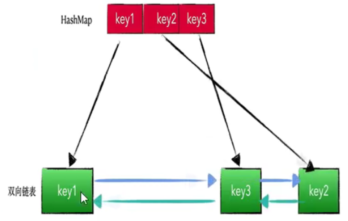
解法二：使用HashMap+双向链表自己写一个。利用了Map的快速查找以及双向链表的快速增删功能，能够实现时间复杂度为O(1)。

public class LRUCache {
    class Node<K, V> {
        K key;
        V value;
        Node<K, V> prev;
        Node<K, V> next;

        public Node() {
            this.prev = this.next = null;
        }

        public Node(K key, V value) {
            this.key = key;
            this.value = value;
            this.prev = this.next = null;
        }
    }

    // 构造一个虚拟的双向链表，它里面包含一个个Node节点作为数据载体
    class DoubleLinkedList<K, V> {
        Node<K, V> head;
        Node<K, V> tail;

        public DoubleLinkedList() {
            head = new Node<>();
            tail = new Node<>();
            head.next = tail;
            tail.prev = head;
        }

        // 添加到头部
        public void addHead(Node<K, V> node) {
            node.next = head.next;
            node.prev = head;
            head.next.prev = node;
            head.next = node;
        }

        // 删除节点
        public void removeNode(Node<K, V> node) {
            node.next.prev = node.prev;
            node.prev.next = node.next;
            node.prev = null;
            node.next = null;
        }

        // 获取最后一个节点
        public Node getLast() {
            return tail.prev;
        }
    }

    private int capacity;
    // map负责查找
    Map<Integer, Node<Integer, Integer>> map;
    // 新建双向链表，头节点放最新访问的节点
    DoubleLinkedList<Integer, Integer> doubleLinkedList;

    public LRUCache(int capacity) {
        this.capacity = capacity;
        map = new HashMap<>();
        doubleLinkedList = new DoubleLinkedList<>();
    }

    public int get(int key) {
        if (!map.containsKey(key)) {
            return -1;
        }
        Node<Integer, Integer> node = map.get(key);
        doubleLinkedList.removeNode(node);
        doubleLinkedList.addHead(node);
        return node.value;
    }

    public void put(int key, int value) {
        if (map.containsKey(key)) {
            Node<Integer, Integer> node = map.get(key);
            node.value = value;
            map.put(key, node);
            doubleLinkedList.removeNode(node);
            doubleLinkedList.addHead(node);
        } else {
            // 容量满了
            if (map.size() == capacity) {
                Node<Integer, Integer> lastNode = doubleLinkedList.getLast();
                map.remove(lastNode.key);
                doubleLinkedList.removeNode(lastNode);
            }
            Node<Integer, Integer> newNode = new Node<>(key, value);
            map.put(key, newNode);
            doubleLinkedList.addHead(newNode);
        }
    }
}

3.2 LFU算法

LFU（Least Frequently Used）算法]根据数据的历史访问频率来淘汰数据，其核心思想是”如果数据过去被访问多次，那么将来被访问的频率也更高”。

要求实现LFUCache类：

LFUCache(int capacity)：用数据结构的容量capacity初始化对象。
int get(int key)：如果键存在于缓存中，则获取键的值，否则返回 -1。
void put(int key, int value)：如果键已存在，则变更其值；如果键不存在，请插入键值对。当缓存达到其容量时，则应该在插入新项之前，使最不经常使用的项无效。在此问题中，当存在平局（即两个或更多个键具有相同使用频率）时，应该去除最近最久未使用的键。
[项的使用次数]就是自插入该项以来对其调用get和put函数的次数之和。使用次数会在对应项被移除后置为0。
为了确定最不常使用的键，可以为缓存中的每个键维护一个使用计数器 。使用计数最小的键是最久未使用的键。

当一个键首次插入到缓存中时，它的使用计数器被设置为1(由于put操作)。对缓存中的键执行get或put操作，使用计数器的值将会递增。

public class LFUCache {
    class Node<K, V> {
        K key;
        V value;
        int freq = 1;
        Node<K, V> prev;
        Node<K, V> next;

        public Node() {
            this.prev = this.next = null;
        }

        public Node(K key, V value) {
            this.key = key;
            this.value = value;
            this.prev = this.next = null;
        }
    }

    class DoubleLinkedList<K, V> {
        Node<K, V> head;
        Node<K, V> tail;

        public DoubleLinkedList() {
            head = new Node<>();
            tail = new Node<>();
            head.next = tail;
            tail.prev = head;
        }

        // 添加到头部
        public void addNode(Node<K, V> node) {
            node.next = head.next;
            node.prev = head;
            head.next.prev = node;
            head.next = node;
        }

        // 删除节点
        public void removeNode(Node<K, V> node) {
            node.next.prev = node.prev;
            node.prev.next = node.next;
            node.prev = null;
            node.next = null;
        }

        // 获取最后一个节点
        public Node<K, V> getLast() {
            return tail.prev;
        }
    }

    Map<Integer, Node<Integer, Integer>> cache; // 存储缓存的内容
    Map<Integer, DoubleLinkedList<Integer, Integer>> freqMap; // 存储每个频次对应的双向链表
    int capacity;
    int min; // 存储当前最小频次

    public LFUCache(int capacity) {
        this.capacity = capacity;
        cache = new HashMap<>();
        freqMap = new HashMap<>();
    }

    public int get(int key) {
        if (!cache.containsKey(key)) {
            return -1;
        }
        Node<Integer, Integer> node = cache.get(key);
        freqInc(node);
        return node.value;
    }

    public void put(int key, int value) {
        if (capacity == 0) {
            return;
        }
        if (cache.containsKey(key)) {
            Node<Integer, Integer> node = cache.get(key);
            node.value = value;
            freqInc(node);
        } else {
            // 容量满了
            if (cache.size() == capacity) {
                DoubleLinkedList<Integer, Integer> minFreqLinkedList = freqMap.get(min);
                cache.remove(minFreqLinkedList.getLast().key);
                // 这里不需要维护min, 因为下面add了newNode后min肯定是1
                minFreqLinkedList.removeNode(minFreqLinkedList.getLast());
            }
            Node<Integer, Integer> newNode = new Node<Integer, Integer>(key, value);
            cache.put(key, newNode);
            DoubleLinkedList<Integer, Integer> linkedList = freqMap.get(1);
            if (linkedList == null) {
                linkedList = new DoubleLinkedList<Integer, Integer>();
                freqMap.put(1, linkedList);
            }
            linkedList.addNode(newNode);
            min = 1;
        }
    }

    public void freqInc(Node<Integer, Integer> node) {
        // 从原freq对应的链表里移除, 并更新min
        int freq = node.freq;
        DoubleLinkedList<Integer, Integer> linkedList = freqMap.get(freq);
        linkedList.removeNode(node);
        if (freq == min && linkedList.head.next == linkedList.tail) {
            min = freq + 1;
        }
        // 加入新freq对应的链表
        node.freq++;
        linkedList = freqMap.get(freq + 1);
        if (linkedList == null) {
            linkedList = new DoubleLinkedList<>();
            freqMap.put(freq + 1, linkedList);
        }
        linkedList.addNode(node);
    }
}